README.md

---
license: apache-2.0
task_categories:
- graph-ml
tags:
- horology
size_categories:
- 100K<n<1M
---

# Watch Market Analysis Graph Neural Network Dataset

## Executive Summary

This dataset transforms traditional watch market data into a Graph Neural Network (GNN) structure, specifically designed to capture the complex dynamics of the pre-owned luxury watch market. 
It addresses three key market characteristics that traditional recommendation systems often miss:

- **Condition-Based Value Dynamics**: Captures how a watch's condition influences its market position and value relative to other timepieces
- **Temporal Price Behaviors**: Models non-linear price patterns where certain watches appreciate while others depreciate
- **Inter-Model Relationships**: Maps complex value relationships between different models that transcend traditional brand hierarchies

### Key Statistics
- Total Watches: 284,491
- Total Brands: 28
- Price Range: $50 - $3.2M
- Year Range: 1559-2024

### Primary Use Cases
- Advanced watch recommendation systems
- Market positioning analysis
- Value relationship modeling
- Temporal trend analysis

## Dataset Description

### Data Structure
The dataset is structured as a PyTorch Geometric Data object with three main components:
- Node features tensor (watch attributes)
- Edge index matrix (watch connections)
- Edge attributes (similarity weights)

### Features
Key features include:
- **Brand Embeddings**: 128-dimensional vectors capturing brand identity and market position
- **Material Embeddings**: 64-dimensional vectors for material types and values
- **Movement Embeddings**: 64-dimensional vectors representing technical hierarchies
- **Temporal Features**: 32-dimensional cyclical embeddings for year and seasonal patterns
- **Condition Scores**: Standardized scale (0.5-1.0) based on watch condition
- **Price Features**: Log-transformed and normalized across market segments
- **Physical Attributes**: Standardized measurements in millimeters

### Network Properties
- **Node Connections**: 3-5 edges per watch
- **Similarity Threshold**: 70% minimum similarity for edge creation
- **Edge Weights**: Based on multiple similarity factors:
  - Price (50% influence)
  - Brand similarity
  - Material type
  - Temporal proximity
  - Condition score

### Processing Parameters
- Batch Size: 50 watches per chunk
- Processing Window: 1000 watches
- Edge Generation Batch: 32 watches
- Network Architecture: Combined GCN and GAT layers with 4 attention heads


## Exploratory Data Analysis

### Brand Distribution

![Brand Distribution Treemap](https://raw.githubusercontent.com/calicartels/watch-market-gnn-code/main/images/2.png)

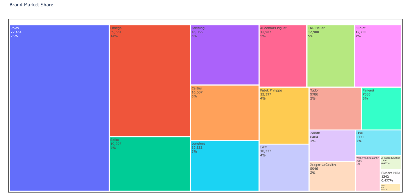
The treemap visualization provides a hierarchical view of market presence:
- Rolex dominates with the highest representation, reflecting its market leadership
- Omega and Seiko follow as major players, indicating a strong market presence
- Distribution reveals clear tiers in the luxury watch market
- Brand representation correlates with market positioning and availability


### Feature Correlations

![Feature Correlation Matrix](https://raw.githubusercontent.com/calicartels/watch-market-gnn-code/main/images/3.png)

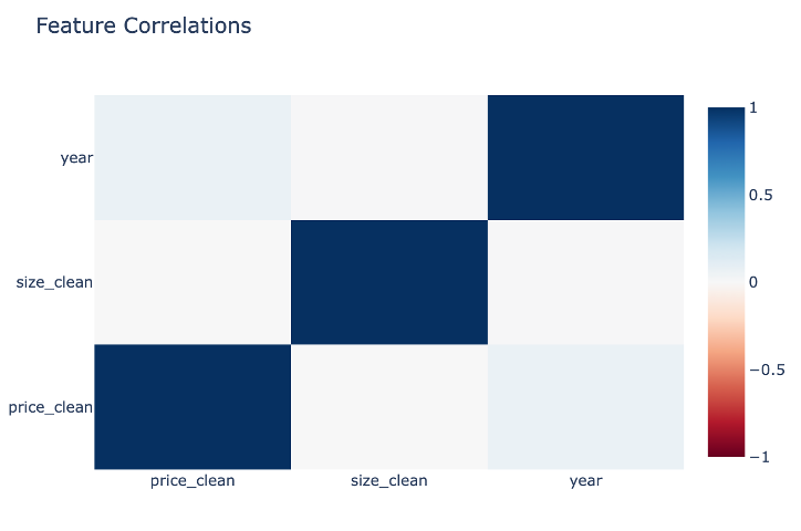
The correlation matrix reveals important market dynamics:
- **Size vs. Year**: Positive correlation indicating a trend toward larger case sizes in modern watches
- **Price vs. Size**: Moderate correlation showing larger watches generally command higher prices
- **Price vs. Year**: Notably low correlation, demonstrating that vintage watches maintain value
- Each feature contributes unique information, validated by the lack of strong correlations across all variables


### Market Structure Visualizations

#### UMAP Analysis

![UMAP Visualization](https://raw.githubusercontent.com/calicartels/watch-market-gnn-code/main/images/4.png)

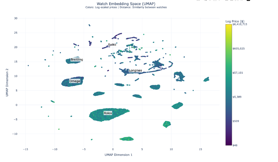
The UMAP visualization unveils complex market positioning dynamics:
- Rolex maintains a dominant central position around coordinates (0, -5), showing unparalleled brand cohesion
- Omega and Breitling cluster in the left segment, indicating strategic market alignment
- Seiko and Longines occupy the upper-right quadrant, reflecting distinct value propositions
- Premium timepieces (yellower/greener hues) show tighter clustering, suggesting standardized luxury attributes
- Smaller, specialized clusters indicate distinct horological collections and style categories


#### t-SNE Visualization

![t-SNE Analysis](https://raw.githubusercontent.com/calicartels/watch-market-gnn-code/main/images/5.png)

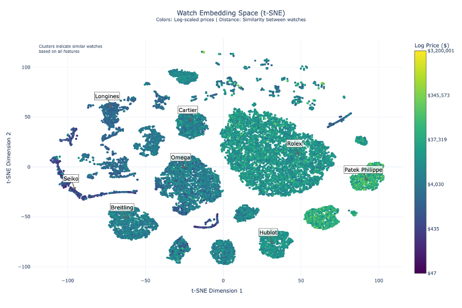
T-SNE analysis reveals clear market stratification with logarithmic pricing from $50 to $3.2M:
- **Entry-Level Segment ($50-$4,000)**
 - Anchored by Seiko in the left segment
 - High volume, accessible luxury positioning
- **Mid-Range Segment ($4,000-$35,000)**
 - Occupies central space
 - Shows competitive positioning between brands
 - Cartier demonstrates strategic positioning between luxury and mid-range
- **Ultra-Luxury Segment ($35,000-$3.2M)**
 - Dominated by Patek Philippe and Audemars Piguet
 - Clear separation in the right segment
 - Strong brand clustering indicating market alignment

#### PCA Analysis

![PCA Visualization](https://raw.githubusercontent.com/calicartels/watch-market-gnn-code/main/images/6.png)

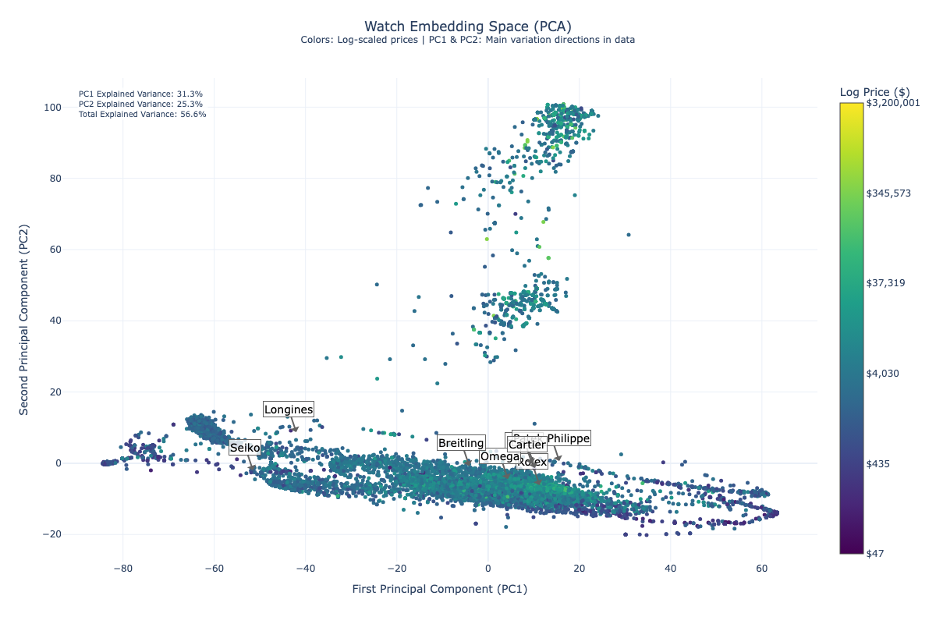
Principal Component Analysis provides robust market insights with 56.6% total explained variance:
- **First Principal Component (31.3%)**
 - Predominantly captures price dynamics
 - Shows clear separation between market segments
- **Second Principal Component (25.3%)**
 - Reflects brand positioning and design philosophies
 - Reveals vertical dispersion indicating intra-brand diversity
- **Brand Trajectory**
 - Natural progression from Seiko through Longines, Breitling, and Omega
 - Culminates in Rolex and Patek Philippe
 - Diagonal trend line serves as a market positioning indicator
- **Market Implications**
 - Successful brands occupy optimal positions along both dimensions
 - Clear differentiation between adjacent competitors
 - Evidence of strategic market positioning


#### Network Visualizations


**Force-Directed Graph**

![Force-Directed Graph](https://raw.githubusercontent.com/calicartels/watch-market-gnn-code/main/images/7.png)

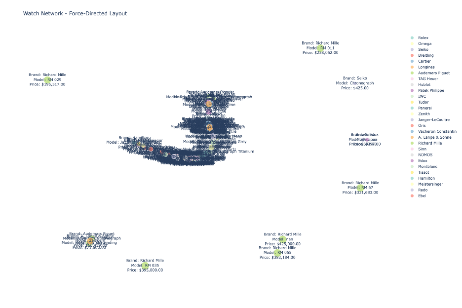
The force-directed layout reveals natural market clustering:
- Richard Mille's peripheral positioning highlights ultra-luxury strategy
- Dense central clustering shows mainstream luxury brand interconnectivity
- Edge patterns reveal shared market characteristics
- Node proximity indicates competitive positioning


**Starburst Visualization**

![Starburst Graph](https://raw.githubusercontent.com/calicartels/watch-market-gnn-code/main/images/8.png)

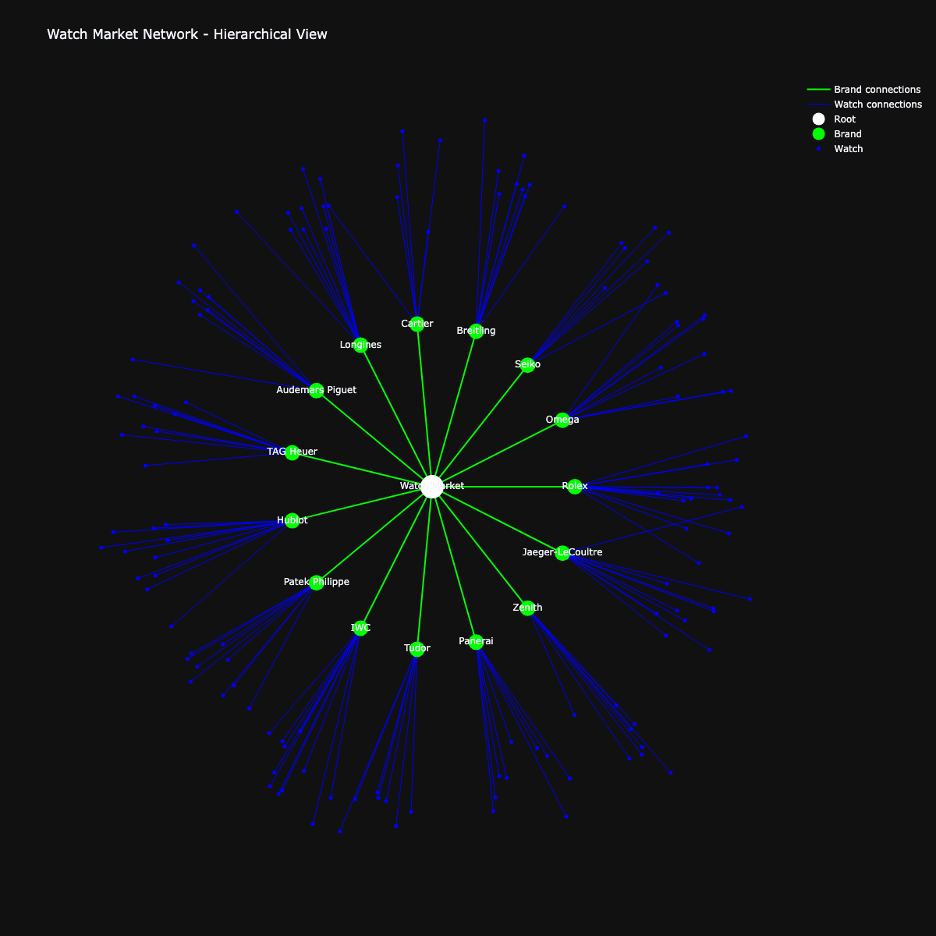
Radial architecture provides a hierarchical market perspective:
- Central node represents the overall market
- Green nodes show brand territories with strategic spacing
- Blue peripheral nodes indicate individual timepieces
- Node density reveals:
 - Brand portfolio breadth
 - Market penetration depth
 - Segment diversification
- Balanced spacing between brand nodes indicates market segmentation


## Ethics and Limitations

### Data Collection and Privacy
- Dataset consists of publicly available watch listings
- No personal information, seller details, or private transaction data
- Serial numbers and identifying marks removed
- Strict privacy standards maintained throughout collection

### Known Biases

#### Connection Strength Bias
- Edge weights and connections based on author's domain expertise
- Similarity thresholds (70%) chosen based on personal market understanding
- Brand value weightings reflect author's market analysis
- Connection strengths may not universally reflect all market perspectives

#### Market Representation Bias
- Predominantly represents online listings
- May not fully capture private sales and in-person transactions
- Popular brands overrepresented (Rolex 25%, Omega 14%)
- Limited editions and rare pieces underrepresented

#### Temporal Bias
- Stronger representation of recent listings
- Historical data may be underrepresented
- Current market conditions more heavily weighted
- Seasonal variations may affect price patterns

#### Brand and Model Bias
- Skewed toward mainstream luxury brands
- Limited representation of boutique manufacturers
- Popular models have more data points
- Vintage and discontinued models may lack comprehensive data

#### Price Bias
- Asking prices may differ from actual transaction values
- Regional price variations not fully captured
- Currency conversion effects on price relationships
- Market fluctuations may not be fully represented

### Usage Guidelines

#### Appropriate Uses
- Market research and analysis
- Academic research
- Watch relationship modeling
- Price trend studies
- Educational purposes

#### Prohibited Uses
- Price manipulation or market distortion
- Unfair trading practices
- Personal data extraction
- Misleading market analysis
- Anti-competitive practices

### License
This dataset is released under the Apache 2.0 License, which allows:
- Commercial use
- Modification
- Distribution
- Private use

While requiring:
- License and copyright notice
- State changes
- Preserve attributions


## Technical Details

### Power Analysis
Minimum sample requirements based on statistical analysis:
- Basic Network: 10,671 nodes (95% confidence, 3% margin)
- GNN Requirements: 14,400 samples (feature space dimensionality)
- Brand Coverage: 768 watches per brand
- Price Segments: 4,320 watches per segment

Current dataset (284,491 watches) exceeds requirements with:
- 5,000+ samples per major brand
- 50,000+ samples per price segment
- Sufficient network density

### Implementation Details

#### Network Architecture
- 3 GNN layers with residual connections
- 64 hidden channels
- 20% dropout rate
- 4 attention heads
- Learning rate: 0.001

#### Embedding Dimensions
- Brand: 128
- Material: 64
- Movement: 64
- Temporal: 32

#### Network Parameters
- Connections per watch: 3-5
- Similarity threshold: 70%
- Batch size: 50 watches
- Processing window: 1000 watches

#### Condition Scoring
- New: 1.0
- Unworn: 0.95
- Very Good: 0.8
- Good: 0.7
- Fair: 0.5

## Usage

### Required Files
The dataset consists of three main files:
- `watch_gnn_data.pt` (315 MB): Main PyTorch Geometric data object
- `edges.npz` (20.5 MB): Edge information
- `features.npy` (596 MB): Node features

### Loading the Dataset

```python
import torch
from torch_geometric.data import Data

# Load the main dataset
data = torch.load('watch_gnn_data.pt')
```

#### Access components

```
node_features = data.x  # Shape: [284491, combined_embedding_dim]
edge_index = data.edge_index  # Shape: [2, num_edges]
edge_attr = data.edge_attr  # Shape: [num_edges, 1]
```
#### For direct feature access
```
features = np.load('features.npy')
```
#### Get number of nodes
```
num_nodes = data.num_nodes
```

#### Get number of edges
```
num_edges = data.num_edges
```

#### Find similar watches (k-nearest neighbors)
```
def find_similar_watches(watch_id, k=5):
    # Get watch features
    watch_features = data.x[watch_id]
    
    # Calculate similarities
    similarities = torch.cosine_similarity(
        watch_features.unsqueeze(0),
        data.x,
        dim=1
    )
    
    # Get top k similar watches
    _, indices = similarities.topk(k+1)  # +1 to exclude self
    return indices[1:]  # Exclude self

# Get watch features
def get_watch_features(watch_id):
    return data.x[watch_id]

```

## Note
- The dataset is optimized for PyTorch Geometric operations
- Recommended to use GPU for large-scale operations
- Consider batch processing for memory efficiency