|
--- |
|
license: apache-2.0 |
|
task_categories: |
|
- graph-ml |
|
tags: |
|
- horology |
|
size_categories: |
|
- 100K<n<1M |
|
--- |
|
|
|
# Watch Market Analysis Graph Neural Network Dataset |
|
|
|
## Executive Summary |
|
|
|
This dataset transforms traditional watch market data into a Graph Neural Network (GNN) structure, specifically designed to capture the complex dynamics of the pre-owned luxury watch market. |
|
It addresses three key market characteristics that traditional recommendation systems often miss: |
|
|
|
- **Condition-Based Value Dynamics**: Captures how a watch's condition influences its market position and value relative to other timepieces |
|
- **Temporal Price Behaviors**: Models non-linear price patterns where certain watches appreciate while others depreciate |
|
- **Inter-Model Relationships**: Maps complex value relationships between different models that transcend traditional brand hierarchies |
|
|
|
### Key Statistics |
|
- Total Watches: 284,491 |
|
- Total Brands: 28 |
|
- Price Range: $50 - $3.2M |
|
- Year Range: 1559-2024 |
|
|
|
### Primary Use Cases |
|
- Advanced watch recommendation systems |
|
- Market positioning analysis |
|
- Value relationship modeling |
|
- Temporal trend analysis |
|
|
|
## Dataset Description |
|
|
|
### Data Structure |
|
The dataset is structured as a PyTorch Geometric Data object with three main components: |
|
- Node features tensor (watch attributes) |
|
- Edge index matrix (watch connections) |
|
- Edge attributes (similarity weights) |
|
|
|
### Features |
|
Key features include: |
|
- **Brand Embeddings**: 128-dimensional vectors capturing brand identity and market position |
|
- **Material Embeddings**: 64-dimensional vectors for material types and values |
|
- **Movement Embeddings**: 64-dimensional vectors representing technical hierarchies |
|
- **Temporal Features**: 32-dimensional cyclical embeddings for year and seasonal patterns |
|
- **Condition Scores**: Standardized scale (0.5-1.0) based on watch condition |
|
- **Price Features**: Log-transformed and normalized across market segments |
|
- **Physical Attributes**: Standardized measurements in millimeters |
|
|
|
### Network Properties |
|
- **Node Connections**: 3-5 edges per watch |
|
- **Similarity Threshold**: 70% minimum similarity for edge creation |
|
- **Edge Weights**: Based on multiple similarity factors: |
|
- Price (50% influence) |
|
- Brand similarity |
|
- Material type |
|
- Temporal proximity |
|
- Condition score |
|
|
|
### Processing Parameters |
|
- Batch Size: 50 watches per chunk |
|
- Processing Window: 1000 watches |
|
- Edge Generation Batch: 32 watches |
|
- Network Architecture: Combined GCN and GAT layers with 4 attention heads |
|
|
|
|
|
## Exploratory Data Analysis |
|
|
|
### Brand Distribution |
|
|
|
 |
|
|
|
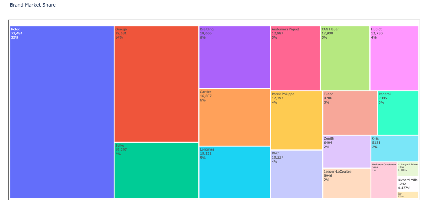
The treemap visualization provides a hierarchical view of market presence: |
|
- Rolex dominates with the highest representation, reflecting its market leadership |
|
- Omega and Seiko follow as major players, indicating a strong market presence |
|
- Distribution reveals clear tiers in the luxury watch market |
|
- Brand representation correlates with market positioning and availability |
|
|
|
|
|
### Feature Correlations |
|
|
|
 |
|
|
|
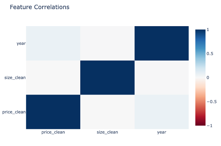
The correlation matrix reveals important market dynamics: |
|
- **Size vs. Year**: Positive correlation indicating a trend toward larger case sizes in modern watches |
|
- **Price vs. Size**: Moderate correlation showing larger watches generally command higher prices |
|
- **Price vs. Year**: Notably low correlation, demonstrating that vintage watches maintain value |
|
- Each feature contributes unique information, validated by the lack of strong correlations across all variables |
|
|
|
|
|
### Market Structure Visualizations |
|
|
|
#### UMAP Analysis |
|
|
|
 |
|
|
|
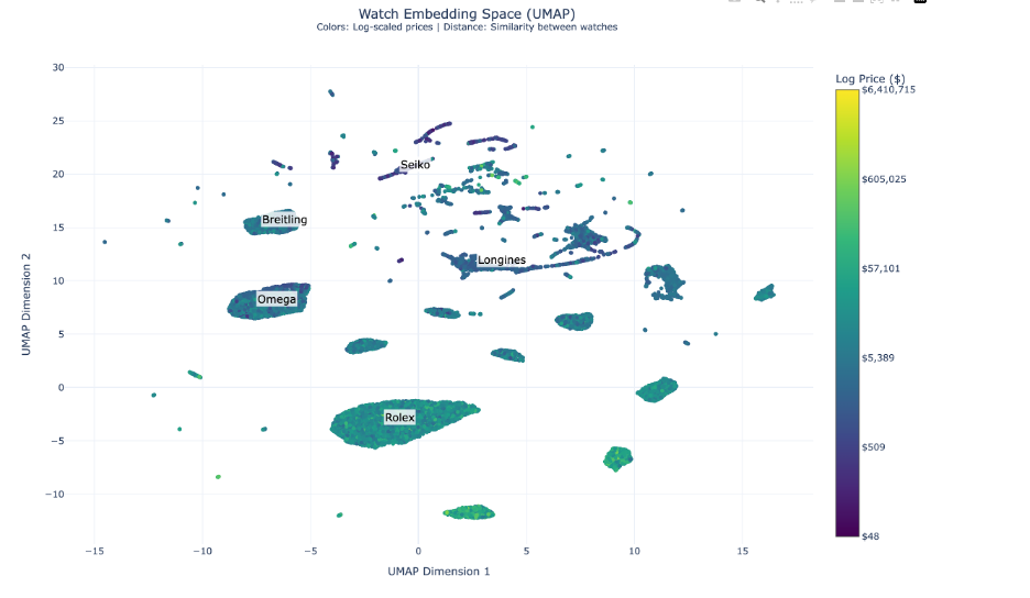
The UMAP visualization unveils complex market positioning dynamics: |
|
- Rolex maintains a dominant central position around coordinates (0, -5), showing unparalleled brand cohesion |
|
- Omega and Breitling cluster in the left segment, indicating strategic market alignment |
|
- Seiko and Longines occupy the upper-right quadrant, reflecting distinct value propositions |
|
- Premium timepieces (yellower/greener hues) show tighter clustering, suggesting standardized luxury attributes |
|
- Smaller, specialized clusters indicate distinct horological collections and style categories |
|
|
|
|
|
#### t-SNE Visualization |
|
|
|
 |
|
|
|
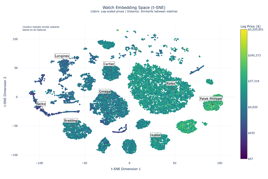
T-SNE analysis reveals clear market stratification with logarithmic pricing from $50 to $3.2M: |
|
- **Entry-Level Segment ($50-$4,000)** |
|
- Anchored by Seiko in the left segment |
|
- High volume, accessible luxury positioning |
|
- **Mid-Range Segment ($4,000-$35,000)** |
|
- Occupies central space |
|
- Shows competitive positioning between brands |
|
- Cartier demonstrates strategic positioning between luxury and mid-range |
|
- **Ultra-Luxury Segment ($35,000-$3.2M)** |
|
- Dominated by Patek Philippe and Audemars Piguet |
|
- Clear separation in the right segment |
|
- Strong brand clustering indicating market alignment |
|
|
|
#### PCA Analysis |
|
|
|
 |
|
|
|
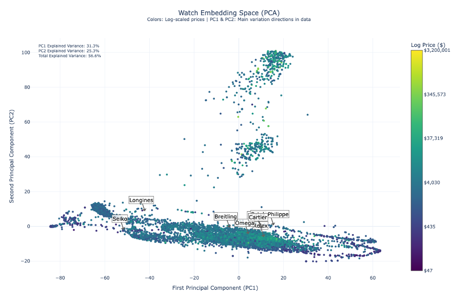
Principal Component Analysis provides robust market insights with 56.6% total explained variance: |
|
- **First Principal Component (31.3%)** |
|
- Predominantly captures price dynamics |
|
- Shows clear separation between market segments |
|
- **Second Principal Component (25.3%)** |
|
- Reflects brand positioning and design philosophies |
|
- Reveals vertical dispersion indicating intra-brand diversity |
|
- **Brand Trajectory** |
|
- Natural progression from Seiko through Longines, Breitling, and Omega |
|
- Culminates in Rolex and Patek Philippe |
|
- Diagonal trend line serves as a market positioning indicator |
|
- **Market Implications** |
|
- Successful brands occupy optimal positions along both dimensions |
|
- Clear differentiation between adjacent competitors |
|
- Evidence of strategic market positioning |
|
|
|
|
|
#### Network Visualizations |
|
|
|
|
|
**Force-Directed Graph** |
|
|
|
 |
|
|
|
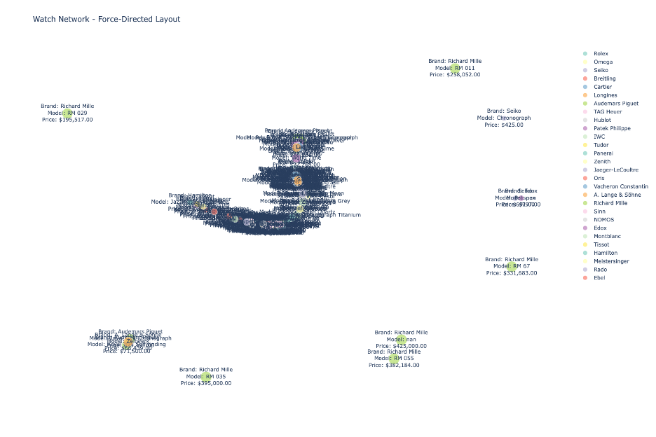
The force-directed layout reveals natural market clustering: |
|
- Richard Mille's peripheral positioning highlights ultra-luxury strategy |
|
- Dense central clustering shows mainstream luxury brand interconnectivity |
|
- Edge patterns reveal shared market characteristics |
|
- Node proximity indicates competitive positioning |
|
|
|
|
|
**Starburst Visualization** |
|
|
|
 |
|
|
|
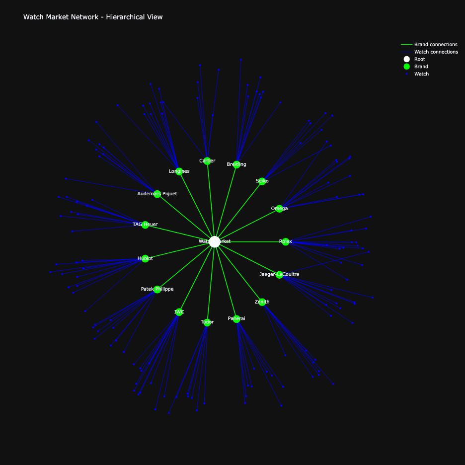
Radial architecture provides a hierarchical market perspective: |
|
- Central node represents the overall market |
|
- Green nodes show brand territories with strategic spacing |
|
- Blue peripheral nodes indicate individual timepieces |
|
- Node density reveals: |
|
- Brand portfolio breadth |
|
- Market penetration depth |
|
- Segment diversification |
|
- Balanced spacing between brand nodes indicates market segmentation |
|
|
|
|
|
## Ethics and Limitations |
|
|
|
### Data Collection and Privacy |
|
- Dataset consists of publicly available watch listings |
|
- No personal information, seller details, or private transaction data |
|
- Serial numbers and identifying marks removed |
|
- Strict privacy standards maintained throughout collection |
|
|
|
### Known Biases |
|
|
|
#### Connection Strength Bias |
|
- Edge weights and connections based on author's domain expertise |
|
- Similarity thresholds (70%) chosen based on personal market understanding |
|
- Brand value weightings reflect author's market analysis |
|
- Connection strengths may not universally reflect all market perspectives |
|
|
|
#### Market Representation Bias |
|
- Predominantly represents online listings |
|
- May not fully capture private sales and in-person transactions |
|
- Popular brands overrepresented (Rolex 25%, Omega 14%) |
|
- Limited editions and rare pieces underrepresented |
|
|
|
#### Temporal Bias |
|
- Stronger representation of recent listings |
|
- Historical data may be underrepresented |
|
- Current market conditions more heavily weighted |
|
- Seasonal variations may affect price patterns |
|
|
|
#### Brand and Model Bias |
|
- Skewed toward mainstream luxury brands |
|
- Limited representation of boutique manufacturers |
|
- Popular models have more data points |
|
- Vintage and discontinued models may lack comprehensive data |
|
|
|
#### Price Bias |
|
- Asking prices may differ from actual transaction values |
|
- Regional price variations not fully captured |
|
- Currency conversion effects on price relationships |
|
- Market fluctuations may not be fully represented |
|
|
|
### Usage Guidelines |
|
|
|
#### Appropriate Uses |
|
- Market research and analysis |
|
- Academic research |
|
- Watch relationship modeling |
|
- Price trend studies |
|
- Educational purposes |
|
|
|
#### Prohibited Uses |
|
- Price manipulation or market distortion |
|
- Unfair trading practices |
|
- Personal data extraction |
|
- Misleading market analysis |
|
- Anti-competitive practices |
|
|
|
### License |
|
This dataset is released under the Apache 2.0 License, which allows: |
|
- Commercial use |
|
- Modification |
|
- Distribution |
|
- Private use |
|
|
|
While requiring: |
|
- License and copyright notice |
|
- State changes |
|
- Preserve attributions |
|
|
|
|
|
## Technical Details |
|
|
|
### Power Analysis |
|
Minimum sample requirements based on statistical analysis: |
|
- Basic Network: 10,671 nodes (95% confidence, 3% margin) |
|
- GNN Requirements: 14,400 samples (feature space dimensionality) |
|
- Brand Coverage: 768 watches per brand |
|
- Price Segments: 4,320 watches per segment |
|
|
|
Current dataset (284,491 watches) exceeds requirements with: |
|
- 5,000+ samples per major brand |
|
- 50,000+ samples per price segment |
|
- Sufficient network density |
|
|
|
### Implementation Details |
|
|
|
#### Network Architecture |
|
- 3 GNN layers with residual connections |
|
- 64 hidden channels |
|
- 20% dropout rate |
|
- 4 attention heads |
|
- Learning rate: 0.001 |
|
|
|
#### Embedding Dimensions |
|
- Brand: 128 |
|
- Material: 64 |
|
- Movement: 64 |
|
- Temporal: 32 |
|
|
|
#### Network Parameters |
|
- Connections per watch: 3-5 |
|
- Similarity threshold: 70% |
|
- Batch size: 50 watches |
|
- Processing window: 1000 watches |
|
|
|
#### Condition Scoring |
|
- New: 1.0 |
|
- Unworn: 0.95 |
|
- Very Good: 0.8 |
|
- Good: 0.7 |
|
- Fair: 0.5 |
|
|
|
## Usage |
|
|
|
### Required Files |
|
The dataset consists of three main files: |
|
- `watch_gnn_data.pt` (315 MB): Main PyTorch Geometric data object |
|
- `edges.npz` (20.5 MB): Edge information |
|
- `features.npy` (596 MB): Node features |
|
|
|
### Loading the Dataset |
|
|
|
```python |
|
import torch |
|
from torch_geometric.data import Data |
|
|
|
# Load the main dataset |
|
data = torch.load('watch_gnn_data.pt') |
|
``` |
|
|
|
#### Access components |
|
|
|
``` |
|
node_features = data.x # Shape: [284491, combined_embedding_dim] |
|
edge_index = data.edge_index # Shape: [2, num_edges] |
|
edge_attr = data.edge_attr # Shape: [num_edges, 1] |
|
``` |
|
#### For direct feature access |
|
``` |
|
features = np.load('features.npy') |
|
``` |
|
#### Get number of nodes |
|
``` |
|
num_nodes = data.num_nodes |
|
``` |
|
|
|
#### Get number of edges |
|
``` |
|
num_edges = data.num_edges |
|
``` |
|
|
|
#### Find similar watches (k-nearest neighbors) |
|
``` |
|
def find_similar_watches(watch_id, k=5): |
|
# Get watch features |
|
watch_features = data.x[watch_id] |
|
|
|
# Calculate similarities |
|
similarities = torch.cosine_similarity( |
|
watch_features.unsqueeze(0), |
|
data.x, |
|
dim=1 |
|
) |
|
|
|
# Get top k similar watches |
|
_, indices = similarities.topk(k+1) # +1 to exclude self |
|
return indices[1:] # Exclude self |
|
|
|
# Get watch features |
|
def get_watch_features(watch_id): |
|
return data.x[watch_id] |
|
|
|
``` |
|
|
|
## Note |
|
- The dataset is optimized for PyTorch Geometric operations |
|
- Recommended to use GPU for large-scale operations |
|
- Consider batch processing for memory efficiency |
|
|